Borrow Interest Rate

Velocity’s lending pools use a borrow interest rate model inspired by Aave . Each spot market defines:

A minimum rate R_min
An optimal rate R_opt at a target utilization U*
A maximum rate R_max at full utilization

The borrow interest rate is a function of utilization (U), or how much capital in the pool is currently lent out.

Utilization Rate and Liquidity

If U is high -> most of the pool is already lent out, so free liquidity is scarce; the protocol charges higher interest rates to incentivise repayment of debt and attract new deposits.
If U is low -> most of the pool is sitting idle and liquidity is abundant; the protocol charges lower interest rates to encourage borrowing.

Multi-Kink Interest Rate Model

To balance capital efficiency with liquidity protection, Velocity uses a multi-kink model. This allows linear rates up to the optimal utilization point, and then introduces increasingly steeper rate hikes as utilization increases, especially in the 85–100% range.

This design allows for more aggressive max utilization rates while not adding too much rate volatility near optimal rate.

Formula

The interest rate function is defined as:

\begin{aligned} &U^*=\frac{\text{optimalUtilization}}{\text{SPOT\_MARKET\_UTILIZATION\_PRECISION}},\quad \Delta R = R_{\max} - R_{\rm opt},\\[0.5em] &R(U)=\max\{R_{\min},\,R_{\rm raw}(U)\},\\[0.5em] &R_{\rm raw}(U)= \begin{cases} R_{\rm opt}\,\frac{U}{U^*}, &U\le U^*,\\[1em] R_{\rm opt} +\Delta R\,\frac{50}{1000}\,\frac{U - U^*}{0.85 - U^*}, &U^*<U\le0.85,\\[1em] R_{\rm opt} +\Delta R\,\frac{50 + 100\,\frac{U - 0.85}{0.05}}{1000}, &0.85<U\le0.90,\\[1em] R_{\rm opt} +\Delta R\,\frac{50 + 100 + 150\,\frac{U - 0.90}{0.05}}{1000}, &0.90<U\le0.95,\\[1em] R_{\rm opt} +\Delta R\,\frac{50 + 100 + 150 + 200\,\frac{U - 0.95}{0.04}}{1000}, &0.95<U\le0.99,\\[1em] R_{\rm opt} +\Delta R\,\frac{50 + 100 + 150 + 200 + 250\,\frac{U - 0.99}{0.005}}{1000}, &0.99<U\le0.995,\\[1em] R_{\rm opt} +\Delta R\,\frac{50 + 100 + 150 + 200 + 250 + 250\,\frac{U - 0.995}{0.005}}{1000}, &0.995<U\le1. \end{cases} \end{aligned}

Graph

This graph demonstrates the multi-kink interest rate model as configured for the SOL market.

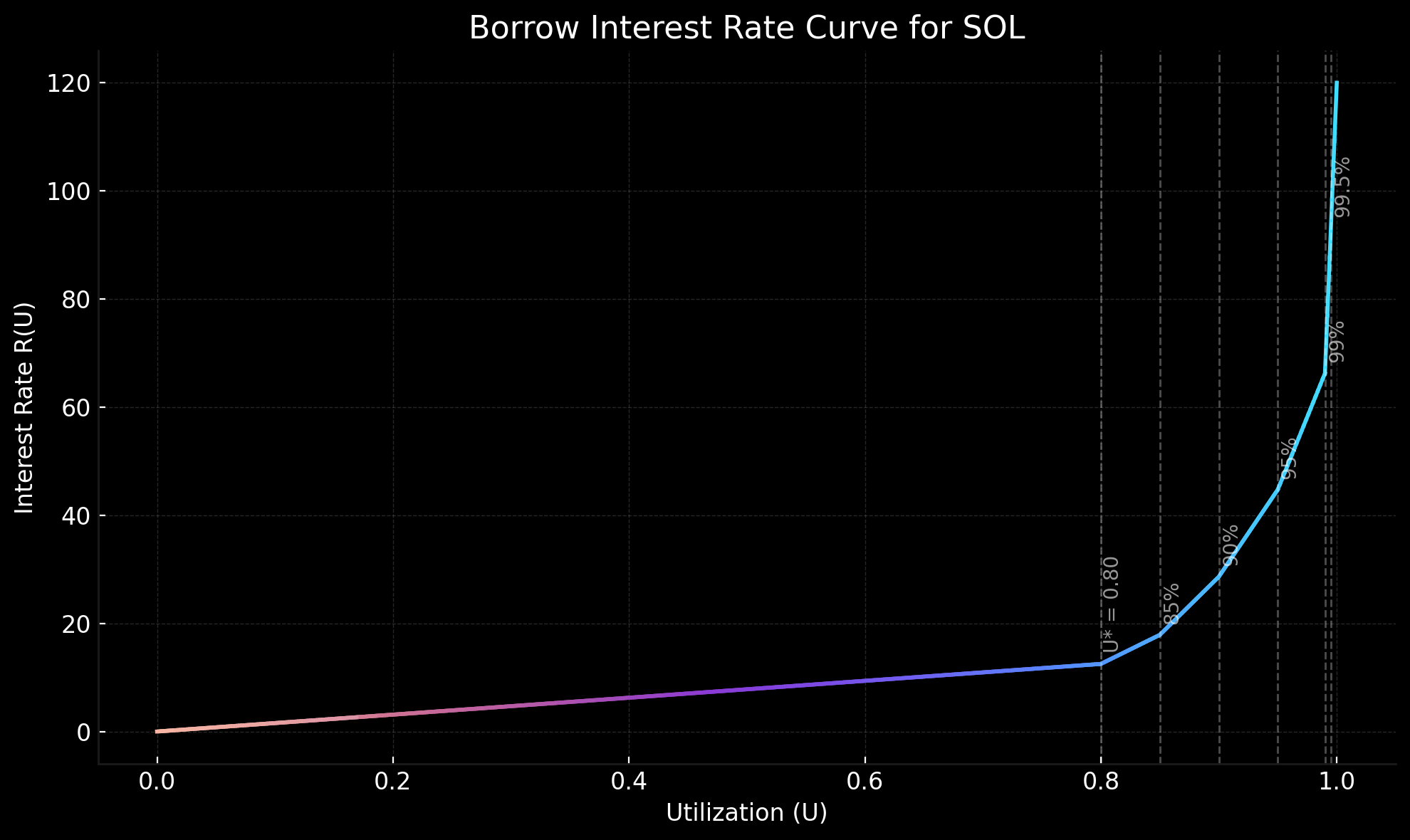
These values are subject to change, as each spot market defines its own parameters. The latest values can be retrieved directly from the on-chain SpotMarketAccount data.

Summary Table

Utilization (U)	Rate Curve Behavior
U ≤ U*	Linear ramp to `R_opt`
U* to 0.85	Mild penalty rate slope(+50 bps)
0.85 to 0.90	Steeper slope (+100 bps)
0.90 to 0.95	Steeper still (+150 bps)
0.95 to 0.99	Aggressive slope (+200 bps)
0.99 to 0.995	Near-vertical slope (+250 bps)
0.995 to 1.00	Max slope (+250 bps)

The multi-kink model and segment weights above are unchanged from the pre-fork Drift Protocol v2 codebase.